【2.4.1.1】tensorflow多GPU的实现-1
欢迎来到本课程的第一个实验。这里的练习有三项目标:
- 复习训练神经网络中用到的基本概念,并为本课程建立通用的术语。
- 阐述神经网络训练中涉及的基本原理(特别是随机梯度下降法)。
- 为本课程的后续实验课打下基础,帮助我们逐步过渡到用多 GPU 实现神经网络。
我们从最简单的神经网络开始,此即单个线性神经元:
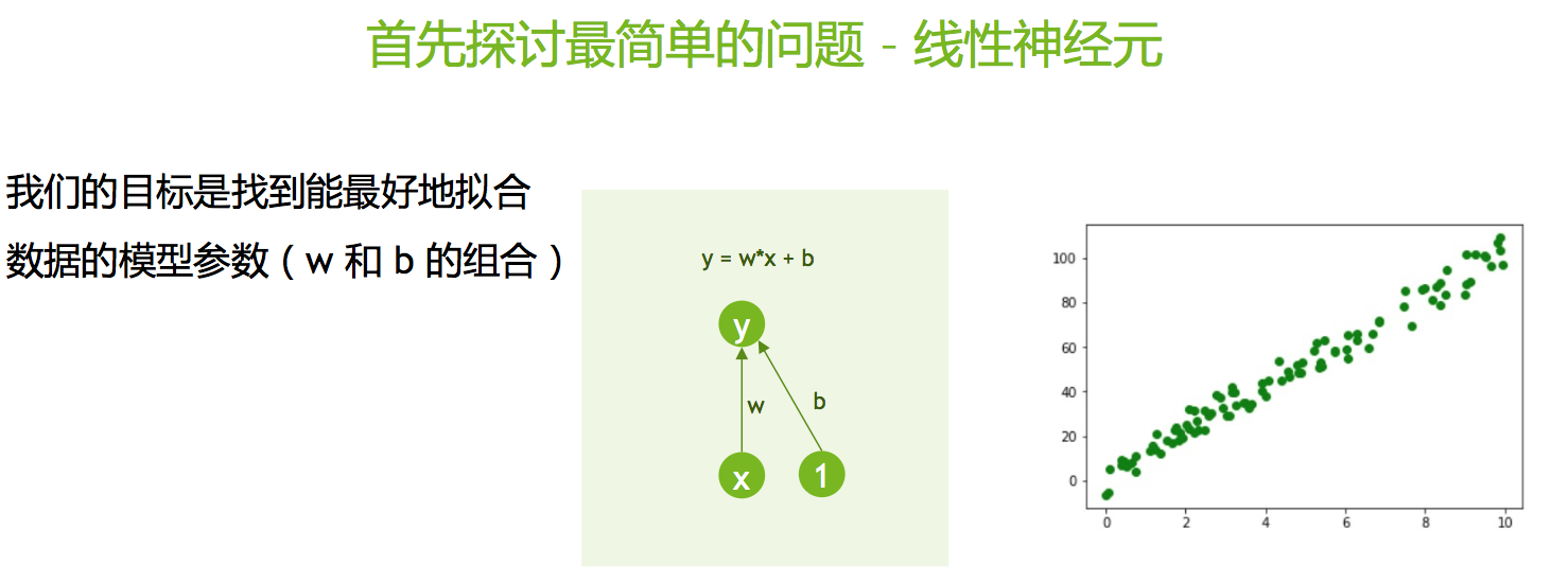
我们将阐述如何使用梯度下降和随机梯度下降算法来训练这一神经网络。
完成本练习后,您将获得对在单个GPU上训练神经网络的理论方面的详细理解。稍后,我们将使用这些知识来说明大规模分布式训练中涉及的所有实际挑战,并重现当代深度神经网络的分布式训练的最新实现技术。
一、训练神经网络
1.1 生成随机数据集
在本练习中,我们将训练我们的神经网络来拟合随机生成的数据点。由于我们的神经网络很简单,它没有太多的预测能力,因此,我们应该生成一个简化的数据集。在本练习中,我们将生成一些呈直线分布的数据点,并添加一定程度的高斯噪声以使问题更贴近于现实。尽管由于存在噪声,直线方程无法完全匹配这些数据点,但它是一个非常好的近似,仍然使我们能够深入研究神经网络的训练过程。
我们首先导入必要的 Python 库。由于这个练习被刻意地简化,所以需要导入的库的数量并不多:
# Numpy is a fundamental package for scientific computing. It contains, among many, an implementation of an array
# that we will use in this exercise.
import numpy as np
# We will be generating our own RANDOM dataset. As a consequence we need functionality to generate random numbers.
import random
# We will be plotting the progress of training as well as the behaviour of our training algorithm
# hence MatPlotLib. A python package that can be used to generate 2D and 3D plots.
import matplotlib.pyplot as plt
# TensorFlow - so the deep learning framework of choice for this class.
import tensorflow as tf
下列变量定义了生成此数据集的属性。我们先从下面给定的值开始(过后您可以随意更改这些值,进而观察噪声对算法性能和算法稳定性的影响)。
# Define the number of samples/data points you want to generate
n_samples = 100
# We will define a dataset that lies on a line as defined by y = w_gen * x + b_gen
w_gen = 10
b_gen = 2
# To make the problem a bit more interesting we will add some Gaussian noise as
# defined by the mean and standard deviation below.
mean_gen = 0
std_gen = 1
# This section generates the training dataset as defined by the variables in the section above.
x = np.float32(np.random.uniform(0, 10, n_samples))
y = np.float32(np.array([w_gen * (x + np.random.normal(loc=mean_gen, scale=std_gen, size=None)) + b_gen for x in x]))
# Plot our randomly generated dataset
plt.close()
plt.plot(x, y, 'go')
plt.xlabel("x", size=24)
plt.ylabel("y", size=24)
plt.tick_params(axis='both', labelsize=16)
plt.tight_layout()
plt.show()
1.2 定义模型
无论机器学习问题有多复杂,代码开发过程都是相同的,包括:
1.创建模型的定义 2. 确定指导我们训练过程的损失函数。损失函数告诉我们,优化算法在模型的训练中取得的进展。它实际上定义了训练成功与否。 3. 然后迭代地进行以下操作:
- 计算损失函数相对于模型权重的梯度。
- 用这个梯度来更新模型权重,以将损失函数最小化。
现在让我们来为一个简单的模型实施上述内容。首先定义模型。
# Define the TensorFlow variables based on our inputs
X = tf.Variable(x, name="X")
Y = tf.Variable(y, name="Y")
# Create our model variables w (weights; this is intended to map to the slope, w_gen) and b (bias; this maps to the intercept, b_gen).
# For simplicity, we initialize the data to zero.
w = tf.Variable(np.float32(0.0), name="weights")
b = tf.Variable(np.float32(0.0), name="bias")
# Define our model. We are implementing a simple linear neuron as per the diagram shown above.
@tf.function
def forward(x):
return w * x + b
1.3 定义损失函数
我们现在必须定义什么是训练成功。我们有很多可用于神经网络的成功衡量指标(亦即损失函数)。如需详细了解可用的损失函数的范围以及如何进行选择,请参阅由 Ian Goodfellow、Yoshua Bengio 和 Aaron Courville 合著的《深度学习》一书的第 6.2.1 节。
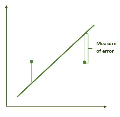
在本例中,我们将使用一个简单的定义。我们将衡量数据集中的所有点与我们试图找到的直线之间的距离的平方之和。
Image
# We define the loss function which is an indicator of how good or bad our model is at any point of time.
loss_fn = tf.keras.losses.MeanSquaredError()
1.4 定义优化逻辑 - 梯度下降
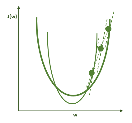
在定义了模型以及损失函数(如模型性能指标)后,下一步是选择优化算法,它能同时找到最小化损失函数(即给予我们最佳性能)的参数 w 和 b 。我们有多种优化算法可供选择(如需更详细的讨论,请参阅《深度学习》一书的第 8 章 )。在本练习中,我们将使用一种最基本的优化算法,即梯度下降法。梯度下降的运行机制如下图所示。请记住:对于非凸函数(如多数神经网络所实现的函数),该算法只会找到局部极小值而非全局极小值。
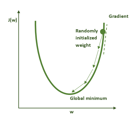
该过程的每一步都使用数据集以及模型参数的当前值(本例中为 w 和 b)来计算使损失函数最小化(即给予我们最佳性能)的梯度(如上图中切线的斜率)。计算出梯度后,可以使用该梯度更新模型参数,使损失函数逐渐向更优解移动。
在实际应用中,我们很少直接使用梯度下降法、甚至下面将讨论的随机梯度下降法的原始形式。相反,现在有它们的更有效的变种,可使算法更快地找到局部最优解,并在计算过程中提供更好的稳定性。其次,梯度计算和优化逻辑代码很少需要从头编写,所有重要的深度学习框架都提供了自动微分以及多种优化算法。在本例中,我们将选择深度学习框架内置的梯度下降优化器。
# Define a gradient descent optimizer
# Note that the "SGD" optimizer is simple gradient descent if applied
# to the full dataset, and stochastic gradient descent if applied to
# random subsets of the dataset
optimizer = tf.keras.optimizers.SGD(learning_rate=0.001)
1.5 训练过程的循环
现在我们已经定义了数据集、模型、损失函数和优化算法,因此我们已准备好开始训练(优化)过程。下面给出的循环将使用整个训练数据集来计算相对于模型参数的损失函数的梯度。然后,每次循环中调用的优化器将对模型参数进行微小的改变(每次改变的大小取决于我们前面设定的学习率),使损失函数愈加接近我们所需的解。我们会将该过程重复足够多次,使此操作最终达到一个合理的解。通常,知道已达到一个好的停止点的方法是损失函数已不再减少。
本练习的目的不仅为讨论分布式随机梯度下降打下基础,还为了解释优化过程的某些属性,这些属性会随着批量的大小(batch size)的增加(由于 GPU 数量的增加)而对算法的性能产生负面影响。为此,在训练时,我们将记录有关训练过程的信息,以便我们能够进一步将该过程可视化。
我们要求您在下面的由TODO指示的代码中完成一个小任务(若不改则该代码不会按原样运行)。 下面的代码块最多可以训练1000次,这远远超过了此问题所需的时间。 请在训练循环内编写代码,使得训练过程在收敛时就能退出循环。收敛是没有通用的定义的,因此您必须选择一个适合此问题的方法。 一种可能的选择是,当损失函数在两次训练的相对变化小于0.1%时就停止训练;您还可以考虑选择模型参数的变化速度。如果遇到困难,可以随时通过修改max_number_of_epochs来消除收敛性检查并控制训练过程。
# Define the maximum number of times we want to process the entire dataset (the number of epochs).
# In practice we won't run this many because we'll implement an early stopping condition that
# detects when the training process has converged.
max_number_of_epochs = 1000
# We will store information about the optimization process here.
loss_array = []
b_array = []
w_array = []
# Zero out the initial values
w.assign(0.0)
b.assign(0.0)
# Print out the parameters and loss before we do any training
Y_predicted = forward(X)
loss_value = loss_fn(Y_predicted, Y)
print("Before training: w = {:4.3f}, b = {:4.3f}, loss = {:7.3f}".format(w.numpy(), b.numpy(), loss_value))
print("")
print("Starting training")
print("")
# Start the training process
for i in range(max_number_of_epochs):
# Use the entire dataset to calculate the gradient and update the parameters
with tf.GradientTape() as tape:
Y_predicted = forward(X)
loss_value = loss_fn(Y_predicted, Y)
optimizer.minimize(loss_value, var_list=[w, b], tape=tape)
# Capture the data that we will use in our visualization
w_array.append(w.numpy())
b_array.append(b.numpy())
loss_array.append(loss_value)
if (i + 1) % 5 == 0:
print("Epoch = {:2d}: w = {:4.3f}, b = {:4.3f}, loss = {:7.3f}".format(i+1, w.numpy(), b.numpy(), loss_value))
# Implement your convergence check here, and exit the training loop if
# you detect that we are converged:
if FIXME: # TODO
break
print("")
print("Training finished after {} epochs".format(i+1))
print("")
print("After training: w = {:4.3f}, b = {:4.3f}, loss = {:7.3f}".format(w.numpy(), b.numpy(), loss_value))
如果您被上面的练习卡住了,请查看下面的单元格里的收敛性检查的示例。
点击这里查看收敛性检查的示例
if i > 1 and abs(loss_array[i] - loss_array[i-1]) / loss_array[i-1] < 0.001:
从下面列出的输出中,我们可以看到我们已设法将损失最大程度地减少到最小,并设法获得了一个离预期的函数足够接近的解(将w和b的当前值与目标值w_gen和b_gen进行比较)。现在,我们将损失作为时间(完成的训练次数)的函数来画损失曲线图。该图是监视训练过程进度的基础,有助于我们了解如何做出改进模型或数据集的重要决策。
plt.close()
plt.plot(loss_array)
plt.xlabel("Epoch", size=24)
plt.ylabel("Loss", size=24)
plt.tick_params(axis='both', labelsize=16)
plt.tight_layout()
plt.show()
1.6 在三维空间中观察模型的损失的运动轨迹
由于本例中的损失函数仅有两个参数(w 和 b),因此创建一个直观易懂的图形来显示其形状是可行的。此外,我们能够对优化算法在其损失函数空间中所走过的轨迹进行可视化。下图说明了这一点
from mpl_toolkits.mplot3d import Axes3D
fig = plt.figure()
ax = fig.gca(projection='3d')
ax.scatter(w_array, b_array, loss_array)
ax.set_xlabel('w', size=16)
ax.set_ylabel('b', size=16)
ax.tick_params(labelsize=12)
plt.show()
现在,我们对上面的可视化进行扩展,画出整个损失函数在这个区域的所有取值。由于我们用整个数据集计算损失函数,我们只获得一个超平面,而且我们的优化器在其上走过的轨迹相当平滑,几乎没有噪声。当我们开始使用数据子集(即批量数据,或部分数据)并开始使用随机梯度下降法进行训练时,情况就变了。
loss_surface = []
w_surface = []
b_surface = []
for w_value in np.linspace(0, 20, 200):
for b_value in np.linspace(-18, 22, 200):
# Collect information about the loss function surface
w.assign(w_value)
b.assign(b_value)
Y_predicted = forward(X)
loss_value = loss_fn(Y_predicted, Y)
b_surface.append(b_value)
w_surface.append(w_value)
loss_surface.append(loss_value)
plt.close()
fig = plt.figure()
ax2 = fig.gca(projection='3d')
ax2.scatter(w_surface, b_surface, loss_surface, c = loss_surface, alpha = 0.02)
ax2.plot(w_array, b_array, loss_array, color='black')
ax2.set_xlabel('w')
ax2.set_ylabel('b')
plt.show()
二、 随机梯度下降法
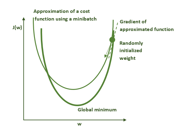
与梯度下降法不同,随机梯度下降法并不使用整个数据集而是使用较小的数据子集(称为一个批次,即batch;其大小称为批量,即batch size)来计算损失函数。这对我们算法的性能有着深远的影响。由于每个批次里的数据是从数据集里随机抽取的,所以每个批次的数据集都不相同。即使对于同一组权重,这些批次的数据集也会提供不同的梯度,引入一定程度的噪声,如下图所示。
下图说明的是过度简化的随机梯度下降算法。粗绿线表示的是用整个数据集计算的损失函数的形状。细绿线表示的是用小批量数据集(亦称minibatch)计算的损失函数的形状。由于这些曲线在本质上有所不同,因此梯度的估计在每一步的计算上都不尽相同,并导致在优化轨迹上产生一定程度的噪声。因此这个方法的名字中有“随机”一词。
第一步
第二步

第三步
如下可知,这种噪声实际上是非常有益的,因为它所产生的极小值的数学特性与梯度下降大相径庭。这在多 GPU 训练问题中之所以重要,是因为通过增加参与训练过程的 GPU 数量,我们实际上加大了批量(batch size),而这会导致减少有益的噪声,这一问题将在今天的第二节课中讲述。
为了证明这种现象,我们对代码做一些细微更改。为了放大随机梯度下降法的效果,我们将仅使用一个样本作为每次迭代中的一个批次的数据,而并非在每次迭代中都向模型提供所有的数据(即把批量从n减至1)。 该过程或者可以被视为产生了一个有效的损失函数,该函数在数学上与完整数据集的损失函数(具有不同的极值)不同,或者可以被视为有助于更好地定位由完整的数据集所计算的损失函数的全局最小值,因为它不太可能陷入局部最小值(我们将在稍后的实际神经网络模型中对此进行研究)。人们可以将梯度下降视为一种算法,可以对所有批次的噪声求平均,而较大批次的噪声要小于较小批次的噪声。 。
2.1 实现随机梯度下降:第一种方法
为了演示这种现象,我们对的代码进行一些小的更改。为了扩大效果 我们在每次迭代中将只提供一个样本(批量大小为1)而不是所有数据给模型。
# Define the maximum number of times we want to process the entire dataset (the number of epochs).
# In practice we won't run this many because we'll implement an early stopping condition that
# detects when the training process has converged.
max_number_of_epochs = 1000
# We will store information about the optimization process here.
loss_array = []
b_array = []
w_array = []
# Zero out the initial values
w.assign(0.0)
b.assign(0.0)
# Print out the parameters and loss before we do any training
Y_predicted = forward(X)
loss_value = loss_fn(Y_predicted, Y)
print("Before training: w = {:4.3f}, b = {:4.3f}, loss = {:7.3f}".format(w.numpy(), b.numpy(), loss_value))
print("")
print("Starting training")
print("")
# Start the training process
for i in range(max_number_of_epochs):
# Update after every data point
for (x_pt, y_pt) in zip(x, y):
with tf.GradientTape() as tape:
y_predicted = forward(x_pt)
loss_value = loss_fn([y_predicted], [y_pt])
optimizer.minimize(loss_value, var_list=[w, b], tape=tape)
# Capture the data that we will use in our visualization
# Note that we are now updating our loss function after
# every point in the sample, so the size of loss_array
# will be greater by a factor of n_samples compared to
# the last exercise.
w_array.append(w.numpy())
b_array.append(b.numpy())
loss_array.append(loss_value)
# At the end of every epoch after the first, print out the learned weights
if i > 0:
avg_w = sum(w_array[(i-1)*n_samples:(i )*n_samples]) / n_samples
avg_b = sum(b_array[(i-1)*n_samples:(i )*n_samples]) / n_samples
avg_loss = sum(loss_array[(i-1)*n_samples:(i )*n_samples]) / n_samples
print("Epoch = {:2d}: w = {:4.3f}, b = {:4.3f}, loss = {:7.3f}".format(i+1, avg_w, avg_b, avg_loss))
# End the training when the loss function has not changed from the last epoch
# by more than a small amount. Note that in our convergence check we will compare
# the loss averaged over this epoch with the loss averaged over the last epoch.
if i > 1:
average_loss_this_epoch = sum(loss_array[(i-1)*n_samples:(i )*n_samples]) / n_samples
average_loss_last_epoch = sum(loss_array[(i-2)*n_samples:(i-1)*n_samples]) / n_samples
if abs(average_loss_this_epoch - average_loss_last_epoch) / average_loss_last_epoch < 0.001:
break
print("")
print("Training finished after {} epochs".format(i+1))
print("")
avg_w = sum(w_array[(i-1)*n_samples:(i )*n_samples]) / n_samples
avg_b = sum(b_array[(i-1)*n_samples:(i )*n_samples]) / n_samples
avg_loss = sum(loss_array[(i-1)*n_samples:(i )*n_samples]) / n_samples
print("After training: w = {:4.3f}, b = {:4.3f}, loss = {:7.3f}".format(avg_w, avg_b, avg_loss))
将最终损失值与我们之前获得的值以及模型参数进行比较。 您可能没有获得相同的总损失值 - 答案是否更准确?
让我们绘制一段时间内的损失。我们可以选择的一种方法是在每次更新后绘制损失。这可能是一条噪声较大的曲线,因为我们没有在整个数据集中遍历所有更新的平均值。
plt.close()
plt.plot(loss_array)
plt.xlabel("Number of Updates", size=24)
plt.ylabel("Loss", size=24)
plt.tick_params(axis='both', labelsize=16)
plt.tight_layout()
plt.show()
此外,绘制我们的优化器在损失函数空间中所走过的轨迹,可以显示大量的噪声。
from mpl_toolkits.mplot3d import Axes3D
plt.close()
fig = plt.figure()
ax = fig.gca(projection='3d')
ax.plot(w_array, b_array, loss_array)
ax.set_xlabel('w', size=16)
ax.set_ylabel('b', size=16)
ax.tick_params(labelsize=12)
plt.show()
绘制一个小批量的损失函数的超平面清楚地表明,它不再与每次生成一个小批量的优化轨迹对齐(对于每个小批量的数据集,它们的损失函数的超平面确实迥异)。
plt.close()
fig = plt.figure()
ax2 = fig.gca(projection='3d')
ax2.scatter(w_surface, b_surface, loss_surface, c = loss_surface, alpha = 0.02)
ax2.plot(w_array, b_array, loss_array, color='black')
ax2.set_xlabel('w')
ax2.set_ylabel('b')
plt.show()
2.2 在最简单的神经网络模型中试验批量大小
我们现在比较两个极端情况:批量数据为完整数据集的随机梯度下降((即传统梯度下降))和批量大小为1的随机梯度下降。让我们尝试一些中间批量值。 为此,请修改我们上面使用的代码,以在每个步骤中传递要训练的数据的子集。 您需要做的就是按顺序遍历数据集,将批量大小为M的每个连续块传递给优化器。
理想情况下,您的实现应适用于任何数量为M的情况,其中1 <= M <= N,其中N是数据集中的样本数。 数据集通常不能被批量大小均匀地整除,因此请确保仅使用所有剩余项来处理数据集中的最后一个批次(因此它将是一个较小的批次)。
# Define the maximum number of times we want to process the entire dataset (the number of epochs).
# In practice we won't run this many because we'll implement an early stopping condition that
# detects when the training process has converged.
max_number_of_epochs = 1000
# We still store information about the optimization process here.
loss_array = []
b_array = []
w_array = []
# Zero out the initial values
w.assign(0.0)
b.assign(0.0)
# Print out the parameters and loss before we do any training
Y_predicted = forward(X)
loss_value = loss_fn(Y_predicted, Y)
print("Before training: w = {:4.3f}, b = {:4.3f}, loss = {:7.3f}".format(w.numpy(), b.numpy(), loss_value))
print("")
print("Starting training")
print("")
# Pass in batches of the dataset
# After the first run, try batch sizes of 16, 64, and 128
batch_size = 32
num_batches_in_epoch = FIXME
# Start the training process
for i in range(max_number_of_epochs):
for j in range(num_batches_in_epoch):
batch_start = FIXME
batch_end = FIXME
with tf.GradientTape() as tape:
y_predicted = forward(x[batch_start:batch_end])
loss_value = loss_fn(y_predicted, y[batch_start:batch_end])
optimizer.minimize(loss_value, var_list=[w, b], tape=tape)
# Capture the data that we will use in our visualization
w_array.append(w.numpy())
b_array.append(b.numpy())
loss_array.append(loss_value)
# At the end of every epoch after the first, print out the learned weights
if i > 0:
avg_w = sum(w_array[(i-1)*num_batches_in_epoch:(i )*num_batches_in_epoch]) / num_batches_in_epoch
avg_b = sum(b_array[(i-1)*num_batches_in_epoch:(i )*num_batches_in_epoch]) / num_batches_in_epoch
avg_loss = sum(loss_array[(i-1)*num_batches_in_epoch:(i )*num_batches_in_epoch]) / num_batches_in_epoch
print("Epoch = {:2d}: w = {:4.3f}, b = {:4.3f}, loss = {:7.3f}".format(i+1, avg_w, avg_b, avg_loss))
# End the training when the loss function has not changed from the last epoch
# by more than a small amount. Note that in our convergence check we will compare
# the loss averaged over this epoch with the loss averaged over the last epoch.
if i > 1:
average_loss_this_epoch = sum(loss_array[(i-1)*num_batches_in_epoch:(i )*num_batches_in_epoch]) / num_batches_in_epoch
average_loss_last_epoch = sum(loss_array[(i-2)*num_batches_in_epoch:(i-1)*num_batches_in_epoch]) / num_batches_in_epoch
if abs(average_loss_this_epoch - average_loss_last_epoch) / average_loss_last_epoch < 0.001:
break
print("")
print("Training finished after {} epochs".format(i+1))
print("")
avg_w = sum(w_array[(i-1)*num_batches_in_epoch:(i )*num_batches_in_epoch]) / num_batches_in_epoch
avg_b = sum(b_array[(i-1)*num_batches_in_epoch:(i )*num_batches_in_epoch]) / num_batches_in_epoch
avg_loss = sum(loss_array[(i-1)*num_batches_in_epoch:(i )*num_batches_in_epoch]) / num_batches_in_epoch
print("After training: w = {:4.3f}, b = {:4.3f}, loss = {:7.3f}".format(avg_w, avg_b, avg_loss))
如果您被上述练习所卡住,请显示下面的单元格以查看示例解决方案。
num_batches_in_epoch = (n_samples + batch_size - 1) // batch_size


...


for j in range(num_batches_in_epoch):
    batch_start = j * batch_size
    batch_end = min((j + 1) * batch_size, n_samples)
现在,对于您尝试的每个批量大小,重复绘图过程以查看运行情况。 请注意哪种批量大小可产生最佳的最终精度,但要特别注意精度曲线的平滑度与训练次数(epochs)的关系,并考虑该平滑度如何取决于批量大小。
plt.close()
plt.plot(loss_array)
plt.xlabel("Number of Updates", size=24)
plt.ylabel("Loss", size=24)
plt.tick_params(axis='both', labelsize=16)
plt.tight_layout()
plt.show()
from mpl_toolkits.mplot3d import Axes3D
plt.close()
fig = plt.figure()
ax = fig.gca(projection='3d')
ax.plot(w_array, b_array, loss_array)
ax.set_xlabel('w', size=16)
ax.set_ylabel('b', size=16)
ax.tick_params(labelsize=12)
plt.show()
plt.close()
fig = plt.figure()
ax2 = fig.gca(projection='3d')
ax2.scatter(w_surface, b_surface, loss_surface, c = loss_surface, alpha = 0.02)
ax2.plot(w_array, b_array, loss_array, color='black')
ax2.set_xlabel('w')
ax2.set_ylabel('b')
plt.show()
三、总结
在这个任务中,我们学到了:
- 神经网络训练过程的基本组成部分
- 如何实现梯度下降优化器
- 梯度下降法和随机梯度下降法之间的差别,以及二者对优化过程的影响
- 批量(batch size)如何影响训练的精度
在本实验课的下一部分中,我们将对上面开发的代码扩展到更大的神经网络,以便可以展示多 GPU 的实现。 在进入下一部分练习(在下一本笔记中)之前,请记得重新启动 IPYTHON 内核来释放已占用的所有 GPU 资源。您可以通过选择“Kernel”(内核)->“Restart”(重启)或运行下列代码来完成。
import IPython
app = IPython.Application.instance()
app.kernel.do_shutdown(True)
参考资料
- Nividia的课件《用多 GPU 训练神经网络》
