【2.4.1.2】tensorflow多GPU的实现-2
更现实的模型
到目前为止,您已经了解了梯度下降(即批量大小等于完整数据集)和小批量随机梯度下降(批量小于完整数据集,通常小得多)之间的区别。 您已经看到较小的批量会在优化过程中增加噪音,而这有助于避免陷入局部最小值或在鞍点处减慢速度。较小的批量也将意味着每一次完整的训练(一个epoch)期间进行多次(更多步)反向传播和梯度更新。

在本实验中,您将在更复杂的数据集和模型上对批量大小进行试验。您将看到批量大小对GPU性能以及训练准确性的影响。
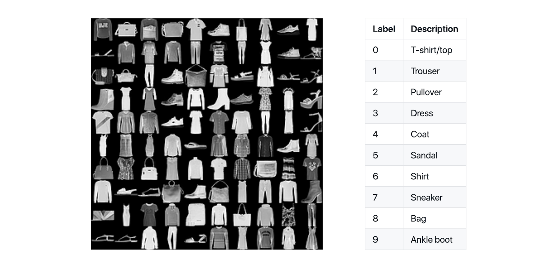
Fashion-MNIST数据集
MNIST数据集通常被称为机器学习里的“hello world”。最初的MNIST数据集包含60,000张手写体数字的图片(0-9)。该数据集的缺点之一是其简单性,一个模型在这个数据集上取得良好性能并不表示该模型将能够在一组更为复杂的图像上表现良好。Fashion-MNIST数据集 是对传统的MNIST数据集的一个回应。
Fashion-MNIST数据集的创建使我们获得一个图像分类方面的中等难度的挑战。 它遵循与原始MNIST集相同的格式,具有10个类别和60,000张28x28像素的图像(加上10,000张测试图像)。 我们将在这个数据集上进行本次模型训练的练习,并在接下来的实验中介绍用多个GPU的模型训练。
宽ResNet模型
我们将使用一个宽残差网络来在该数据集上进行训练。宽残差网络是一个经过证明的在图像分类挑战中表现出色的卷积神经网络。请花一些时间来了解有关宽残差网络、以及最初的残差网络的更多信息,或了解一下卷积神经网络。
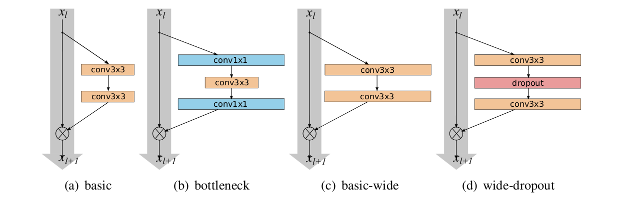
在CNN的早期,深度学习界倾向非常深的模型(数十或数百层)。但是随着计算能力的提高和算法的改进,尤其是在证明了残差块的概念之后,人们更愿意回到具有较宽及较浅层的网络,这种网络是WideResNet模型系列的主要创新。我们将在下面使用的WideResNet-16-10以其千万级的参数所达到的精度可以与有更多参数的更深层网络所达到的精度相媲美。
训练我们的模型
我们将使用默认超参数在现有数据集上开始训练。 请花几分钟浏览一下fashion_mnist.py (入下),并熟悉训练过程。 我们使用Keras进行此训练,但是这些练习的内容可以转化到其它框架上。
import argparse
import tensorflow as tf
from tensorflow.keras import backend as K
from tensorflow.keras.preprocessing import image
from tensorflow.keras.datasets import fashion_mnist
from tensorflow.keras.layers import Input, Conv2D, BatchNormalization, Dense, \
                                    Add, Activation, Dropout, MaxPooling2D, GlobalAveragePooling2D
import numpy as np
import os
from time import time

# Parse input arguments

parser = argparse.ArgumentParser(description='Fashion MNIST Example',
                                 formatter_class=argparse.ArgumentDefaultsHelpFormatter)
parser.add_argument('--log-dir', default='./logs',
                    help='tensorboard log directory')
parser.add_argument('--batch-size', type=int, default=32,
                    help='input batch size for training')
parser.add_argument('--val-batch-size', type=int, default=32,
                    help='input batch size for validation')
parser.add_argument('--epochs', type=int, default=40,
                    help='number of epochs to train')
parser.add_argument('--base-lr', type=float, default=0.01,
                    help='learning rate for a single GPU')
parser.add_argument('--wd', type=float, default=0.000005,
                    help='weight decay')
# TODO Step 2: Add target and patience arguments to the argument parser

args = parser.parse_args()

# Define a function for a simple learning rate decay over time

def lr_schedule(epoch):

    if epoch < 15:
        return args.base_lr
    if epoch < 25:
        return 1e-1 * args.base_lr
    if epoch < 35:
        return 1e-2 * args.base_lr
    return 1e-3 * args.base_lr

# Define the function that creates the model

def cbr(x, conv_size):
    channel_axis = 1 if K.image_data_format() == 'channels_first' else -1

    x = Conv2D(conv_size, (3,3), padding='same')(x)
    x = BatchNormalization(axis=channel_axis)(x)
    x = Activation('relu')(x)

    return x

def conv_block(x, conv_size, scale_input = False):
    x_0 = x
    if scale_input:
        x_0 = Conv2D(conv_size, (1, 1), activation='linear', padding='same')(x_0)

    x = cbr(x, conv_size)
    x = Dropout(0.01)(x)
    x = cbr(x, conv_size)
    x = Add()([x_0, x])

    return x

def create_model():

    # Implementation of WideResNet (depth = 16, width = 10) based on keras_contrib
    # https://github.com/keras-team/keras-contrib/blob/master/keras_contrib/applications/wide_resnet.py

    inputs = Input(shape=(28, 28, 1))

    x = cbr(inputs, 16)

    x = conv_block(x, 160, True)
    x = conv_block(x, 160)
    x = MaxPooling2D((2, 2))(x)
    x = conv_block(x, 320, True)
    x = conv_block(x, 320)
    x = MaxPooling2D((2, 2))(x)
    x = conv_block(x, 640, True)
    x = conv_block(x, 640)
    x = GlobalAveragePooling2D()(x)

    outputs = Dense(num_classes, activation='softmax')(x)

    model = tf.keras.models.Model(inputs, outputs)

    opt = tf.keras.optimizers.SGD(lr=args.base_lr)

    model.compile(loss=tf.keras.losses.categorical_crossentropy,
                  optimizer=opt,
                  metrics=['accuracy'])

    return model

verbose = 1

# Input image dimensions
img_rows, img_cols = 28, 28
num_classes = 10

# Load Fashion MNIST data.
(x_train, y_train), (x_test, y_test) = fashion_mnist.load_data()

# Train only on 1/6 of the dataset
x_train = x_train[:10000,:,:]
y_train = y_train[:10000]

if K.image_data_format() == 'channels_first':
    x_train = x_train.reshape(x_train.shape[0], 1, img_rows, img_cols)
    x_test = x_test.reshape(x_test.shape[0], 1, img_rows, img_cols)
    input_shape = (1, img_rows, img_cols)
else:
    x_train = x_train.reshape(x_train.shape[0], img_rows, img_cols, 1)
    x_test = x_test.reshape(x_test.shape[0], img_rows, img_cols, 1)
    input_shape = (img_rows, img_cols, 1)

# Convert class vectors to binary class matrices
y_train = tf.keras.utils.to_categorical(y_train, num_classes)
y_test = tf.keras.utils.to_categorical(y_test, num_classes)

# Training data iterator.
train_gen = image.ImageDataGenerator(featurewise_center=True, featurewise_std_normalization=True,
                                     horizontal_flip=True, width_shift_range=0.2, height_shift_range=0.2)
train_gen.fit(x_train)
train_iter = train_gen.flow(x_train, y_train, batch_size=args.batch_size)

# Validation data iterator.
test_gen = image.ImageDataGenerator(featurewise_center=True, featurewise_std_normalization=True)
test_gen.mean = train_gen.mean
test_gen.std = train_gen.std
test_iter = test_gen.flow(x_test, y_test, batch_size=args.val_batch_size)


callbacks = []
callbacks.append(tf.keras.callbacks.LearningRateScheduler(lr_schedule))

# TODO Step 1: Define the PrintThroughput callback

# TODO Step 1: Add the PrintThrought callback to the callbacks list

# TODO Step 2: Define the StopAtAccuracy callback

# TODO Step 2: Add the StopAtAccuracy callback to the callbacks list

# TODO Step 3: Define the PrintTotalTime callback

# TODO Step 3: Add the PrintTotalTime callback to the callbacks list

# Create the model.
model = create_model()

# Train the model.
model.fit(train_iter,
          steps_per_epoch=len(train_iter),
          callbacks=callbacks,
          epochs=args.epochs,
          verbose=verbose,
          workers=4,
          initial_epoch=0,
          validation_data=test_iter,
          validation_steps=len(test_iter))

# Evaluate the model on the full data set.
score = model.evaluate(test_iter, steps=len(test_iter), workers=4)
if verbose:
    print('Test loss:', score[0])
    print('Test accuracy:', score[1])
请注意,本练习仅针对1/6的数据集(10,000张图像)进行训练。 我们这样做是为了缩短单次训练的时间,以便我们可以进行快速实验并查看批量大小的影响。当我们开始引入多个GPU来加快训练速度时,我们将使用整个数据集。
在你对代码有了充分了解后,请执行以下单元并训练几次。请注意验证集上的精度、验证损失和每次训练的时间。
!python fashion_mnist.py --epochs 5
我们将对该文件进行一些编辑,因此,让我们对该文件进行备份,以防您出错。
!cp fashion_mnist.py fashion_mnist_original.py
训练的性能 – 图像数/秒
衡量训练效果的一种方法是在给定的单位内时间能处理多少数据。 GPU已针对并行处理进行了高度优化,并且训练过程的许多方面都利用了这种并行性。请花一点时间思考为什么批量大小可能会影响GPU的并行处理能力以及性能可能发生什么变化。
在本练习中,您将实现一个函数,该函数将报告神经网络训练时每秒处理多少图像。然后,您将调整批量大小,并根据经验观察性能(或吞吐量)是如何受到影响的。
实现回调函数(callback)
在我们的训练中,我们将使用自定义的Keras回调函数来报告图像/秒吞吐量。请花时间查看一下fashion_mnist.py中的callbacks/throughput.py以及相应的TODO Step 1位置。将代码复制到fashion_mnist.py中的相应位置。如果遇到问题,可以查看solutions / fashion_mnist_after_step_01.py。
# TODO Step 1: Define the PrintThroughput callback
class PrintThroughput(tf.keras.callbacks.Callback):
    def __init__(self, total_images=0):
        self.total_images = total_images

    def on_epoch_begin(self, epoch, logs=None):
        self.epoch_start_time = time()

    def on_epoch_end(self, epoch, logs={}):
        epoch_time = time() - self.epoch_start_time
        images_per_sec = round(self.total_images / epoch_time, 2)
        print('Images/sec: {}'.format(images_per_sec))

# TODO Step 1: Add the PrintThrought callback to the callbacks list
PrintThroughput(total_images=len(y_train))
一旦实现了回调函数,请再次执行训练过程。 请注意在停止训练前的2~3次训练的吞吐量。
!python fashion_mnist.py --epochs 5
您会注意到,在第一次训练之后吞吐量增加了。这可以归因于单次成本,例如数据加载和内存分配。在下一个练习中,请仅关注第二次及以后训练的吞吐量。
按批量大小比较吞吐量
在本练习中,您将根据批量大小来计算训练吞吐量。调整批量大小时,请多次执行下一个单元格。 在下面的单元格中输入数据(用对应的批量大小的图像/秒吞吐量替换每个“FIXME”),然后执行它以查看数据图。
!python fashion_mnist.py --epochs 5 --batch-size FIXME
%matplotlib widget
import matplotlib.pyplot as plt
data = [('8', FIXME),
('16', FIXME),
('32', FIXME),
('64', FIXME),
('128', FIXME),
('256', FIXME),
('512', FIXME),
('700', FIXME)] # See what happens when you go much above 700
x,y = zip(*data)
plt.bar(x,y)
plt.ylabel("Throughput (images / sec)")
plt.xlabel("Batch Size")
plt.show()
如果您不想手动查找每个数据点,则可以显示下面的代码块并复制我们提供的数据。
data = [('8', 328), ("16", 551), ("32", 808), ("64", 1002), ("128", 1165), ("256", 1273), ("512", 1329), ("700", 1332)]
请花一些时间查看数据并考虑可能发生了什么情况。如果你想到了一些假设的结论,请显示以下方框。
显然,吞吐量随着批量的增加而增加。由于GPU的并行处理特性,这样的结果是合理的。较大的批量意味着更多的图像可以并行地通过模型,以计算反向传播发生前的损失。而这种并行计算利用了GPU中成千上万的内核。
但是,吞吐量不会随批量大小线性地增加,而且随着批量的进一步增加,收益会递减。最终,您将使GPU的计算能力达到饱和点。当GPU可以同时生成数万或数十万个线程时,它们可以更有效率地工作。对于小批量而言,工作量还不足以使GPU使用所有可以执行的线程。由于GPU的处理性能取决于有很多工作要做来隐藏延迟,因此小批量的性能将相对较差;而对于很大的批量,训练的性能终将因用尽所有GPU内核使吞吐量(每秒处理的图像数)接近上限。
训练的性能 – 达到指定准确率的时间
现在,您可能希望选择最大的批量进行训练,以实现最高的吞吐量。但是,尽管吞吐量是训练过程的重要指标,但是它并不能说明模型对实现其目的(即推理)而言被训练得有多好。
在我们的案例中,模型仅具有在给定图像中正确识别服装类别的能力。对模型的准确性的测量是在验证集的准确性上反映的,即模型在我们未用于训练的单独的数据集上进行的预测是否有效。
请仔细考虑批量大小可能会如何影响模型的准确性。请记住,批量较小时引入的噪音是训练过程中的有用工具。
在下一个练习中,您将再次调整批量大小,并比较达到指定精度之前的总的训练时间。
提早中止(Early Stopping)
请花一点时间查看callbacks/early_stopping.py中的代码。 请注意,您对目标精度和耐心值(patience)进行了初始化。 耐心值确定的是,训练在应停止之前有多少次超过了目标准确性。有时,在对网络进行了有效的训练之前,验证准确性可能会意外地急剧上升。在一个以上的连续训练次数内都保持较高的准确性,可以使我们更有把握地相信该网络已受过良好训练,并且可以有效地泛化。
# TODO Step 2: Add target and patience arguments to the argument parser
parser.add_argument('--target-accuracy', type=float, default=.85,
                    help='Target accuracy to stop training')
parser.add_argument('--patience', type=float, default=2,
                    help='Number of epochs that meet target before stopping')

# TODO Step 2: Define the StopAtAccuracy callback
class StopAtAccuracy(tf.keras.callbacks.Callback):
    def __init__(self, target=0.85, patience=2):
        self.target = target
        self.patience = patience
        self.stopped_epoch = 0
        self.met_target = 0

    def on_epoch_end(self, epoch, logs=None):
        if logs.get('val_accuracy') > self.target:
            self.met_target += 1
        else:
            self.met_target = 0

        if self.met_target >= self.patience:
            self.stopped_epoch = epoch
            self.model.stop_training = True

    def on_train_end(self, logs=None):
        if self.stopped_epoch > 0:
            print('Early stopping after epoch {}'.format(self.stopped_epoch + 1))

# TODO Step 2: Add the StopAtAccuracy callback to the callbacks list
StopAtAccuracy(target=args.target_accuracy, patience=args.patience)
请在fashion_mnist.py中寻找TODO Step 2并加入由callbacks/early_stopping.py实现回调函数,以实现提早终止。最后,使用给定的目标精度和耐心值进行以下训练。如果遇到问题,可以查看solutions/fashion_mnist_after_step_02.py。
!python fashion_mnist.py --target-accuracy .82 --patience 2
报告总的训练时间
既然您已经在达到了一定的精度时停止了训练,下一步就是报告总的训练时间,以便您可以相互比较不同轮次的训练。 请仔细阅读callbacks/total_time.py中的代码,并在fashion_mnist.py中寻找TODO Step 3位置加入回调函数。 如果遇到问题,可以查看solutions/fashion_mnist_after_step_03.py。
# TODO Step 3: Define the PrintTotalTime callback
class PrintTotalTime(tf.keras.callbacks.Callback):
    def on_train_begin(self, logs=None):
        self.start_time = time()

    def on_epoch_end(self, epoch, logs=None):
        total_time = round(time() - self.start_time, 2)
        print("Cumulative training time after epoch {}: {}".format(epoch + 1, total_time))

    def on_train_end(self, logs=None):
        total_time = round(time() - self.start_time, 2)
        print("Cumulative training time: {}".format(total_time))

# TODO Step 3: Add the PrintTotalTime callback to the callbacks list
PrintTotalTime()
完成后,请再次运行这个程序以测试功能。这个练习现在可以使用较低的目标精度或较低的耐心阈值,因为我们只想确保我们正确地编写了代码。
!python fashion_mnist.py --target-accuracy FIXME --patience FIXME
比较精度和批量大小
您现在有了一个系统,可以将批量大小对达到某个精度(建议在.82和.85之间)的训练时间的影响进行比较。请多尝试几个批量值,并查看它们对验证精度的影响。请注意当批量太小或太高时会发生什么。请考虑以相同的批量大小重复训练一次或多次,以评估结果的一致性。
!python fashion_mnist.py --batch-size FIXME --target-accuracy FIXME --patience FIXME
在查看下一部分之前,记录并思考您得到的结果。
您获得的结果可能为您提供了两个大致的方向。 特别是,非常小或非常大的批量对于模型训练的收敛来说可能不是最佳选择(非常小的批量带来的噪声往往过于嘈杂而无法使模型充分收敛到损失函数的最小值,而非常大的批量则往往造成训练的早期阶段就发散)。 但是,您可能还看到结果中存在很多随机性,因此很难实现良好的泛化能力。不过这没关系,而且这实际上是一件好事,因为并非您今天学习的所有内容都将以相同的方式应用于每个模型和数据集。本课程的目的是建立关于如何看待神经网络的优化过程的直觉,而不是学习一套盲目地应用于生产的规则。
结论
在本节课中,我们学习了:
- 如何训练比以前使用的模型更复杂、更实际的神经网络模型
- 如何在Keras中实现几个自定义回调函数,并根据精度和吞吐量来衡量训练性能
- 对于更现实的模型,批量大小如何影响训练精度
- 实验1到此结束。在实验2中,我们将学习如何将训练过程扩展到多个GPU。
参考资料
- Nividia的课件《用多 GPU 训练神经网络》
