排序【5】--PCoA主坐标分析

July 09, 2017 gradient 阅读量：次

一、PCoA简介

这是一种排序方法。假设我们对N个样方有了衡量它们之间差异即距离的数据,就可以用此方法找出一个直角坐标系(最多N-1维),使N个样方表示成N个点,而使点间的欧氏距离的平方正好等于原来的差异数据。

主坐标分析是Gower(1966)建立的。因为样方间差异数据可用各种各样的办法给出, 这种方法用得很普遍。例如原来只知样本属甲型、乙型、丙型……等名称的区别,只要对不同型间的差异给以适当的数量描述,就可以用此方法求出各样方的数量坐标,从而实现定性数据的定量转换。

主坐标方法简单、明确、效率很高。它与主分量分析一样,最后找出的坐标系不仅正交, 而且第一轴、第二轴……依次按N个点在该轴上的方差大小顺序排列,N个点对不同两个轴都不相关。所以也可用较少的维数,特别是直观的二、三维空间去排列样方,而使信息的损失最少。它与主分量分析不同之处在于:不是先给出N个点的坐标,去找出刚性旋转的坐标;而是只知其间的距离要去重新建立各点的坐标。因此可以不限于度量(metrtic)的相似系数公式,Pernitec(1977)采用数量数据对于寒温带森林和草地进行主坐标分析,他认为非度量(non-mertic)相似系数比度量相似系数效果更佳。

PCoA这个方法也是MDS (Metric Multidimensional Scaling)。

PCA用的距离矩阵为Euclidean distances，CA用的距离矩阵为chi-square distances，PCoA一般也是用的为Euclidean来表示样品之间的距离关系。同时PCoA也有特征值，用以说明轴的贡献， (This method is also known as MDS (Metric Multidimensional Scaling). While PCA preserves Euclidean distances among samples and CA chi-square distances, PCoA provides Euclidean representation of a set of objects whose relationship is measured by any similarity or distance measure chosen by the user. As well as PCA and CA, PCoA returns a set of orthogonal axes whose importance is measured by eigenvalues. This means that calculating PCoA on Euclidean distances among samples yields the same results as PCA calculated on covariance matrix of the same dataset (if scaling 1 is used).)

NMDS (Non-metric Multidimensional Scaling):

Non-metric alternative to PCoA analysis - it can use any distance measure among samples, and the main focus is on projecting the relative position of sample points into low dimensional ordination space (two or three axes). The method is distance based, not eigenvalue based - it means that it does not attempt to maximize the variance preserved by particular ordination axes and resulting projection could therefore be rotated in any direction.

二、 PCoA分析步骤

主坐标分析的步骤如下:

1)构成样本间差异的数据矩阵M

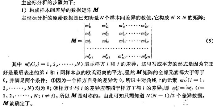
M的数据一般不是生态工作者观察群落的原始记录,而是由原始记录推导出来的,它有各种推导方法。

2)构成离差矩阵A

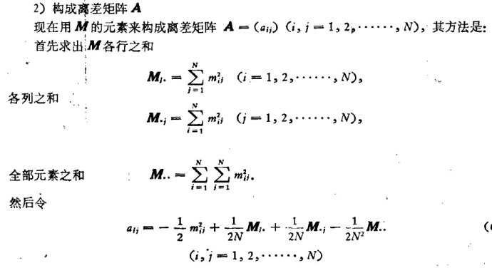
就求出A矩阵的元素。以后可知,它是最后求出的N个样方点坐标矩阵的离差矩阵。这里不必证明而列出A具有的三个性质:1，A是对称的,即aij~aji(i,j=1,2,……,N)2,A的行和及列和均等于0,即Ai.=A.i=0; 3,

mij2=mji2=aii+ajj-2aij( i,j=1,2,……,N).

3)求出N个样方点的坐标矩阵C

因为A是NxN的对称实矩阵,所以必存在着酉矩阵(正交矩阵)U将A变换成对角矩B,即 UAU’=B,或A=U’BU。其中B的主对角线元素为λ1, λ2,……λN，分别是A的N个依大小排列的特征根,而U的每一行向量是相应的特征向量。

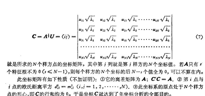
4 ) 排列N个样方

根据C给出的N个样方的坐标值,可以在s维空间中排列样方,而不损失信息。与主分量分析一样 , 可以在较低K(< s)维空间中排列样方, 则保留的信息百分比为 :

$$ \sum _{i=1}^{K}\lambda_{i}/ \sum _{i=1}^{s}\lambda_{i}$$

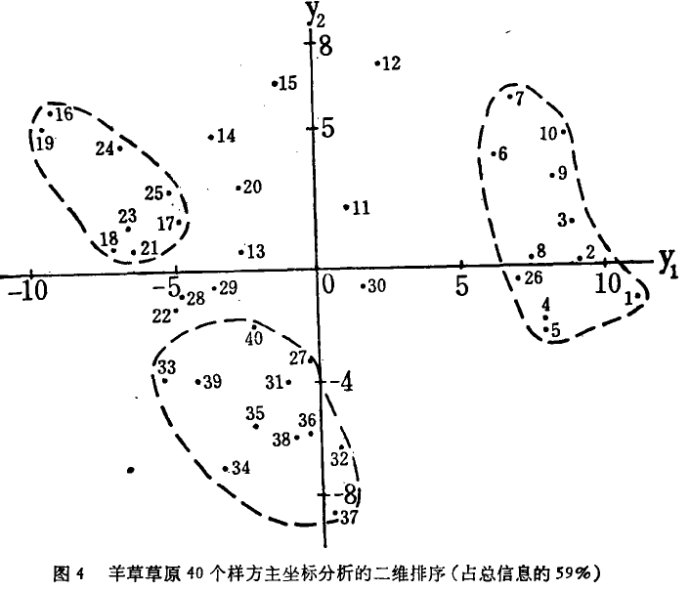
。特别是只选择二、三维主坐标就可直观地画出它们的排序图形

三、PCOA分析

cmdscale( ) stats包
wcmdscale( ) vegan包：加权的经典标度
pco( ),ecodist包
pco( ),labdsv包
pcoa( ),ape包
dudi.pco( ),ade4包：后四种方法采用主坐标分析（经典标度的另一种表述），这几个包和生态，进化，遗传有关。

度量标度：

sammon映射：sammon（），MASS包

非度量标度：

isoMDS（），MASS包

metaMDS（）,vegan包

monoMDS（），vegan包（全局和局部的非度量标度，局部的多维标度在非线性维数缩减部分介绍）

保序回归：

isoreg（），stats包

(2) SMACOF方法和smacof包，复杂MDS问题的求解。

1，vegan包中的cmdscale根据距离矩阵做PCOA分析

spe.bray <- vegdist(spe)#先算距离矩阵
 spe.b.pcoa <- cmdscale(spe.bray, k=(nrow(spe)-1), eig=TRUE) #输入距离矩阵计算PCoA
ordiplot(spe.b.pcoa)
ordiplot来作图
 
city<-read.csv('airline.csv',header=TRUE)
city1<-city[,-1]#这个数据集的第一列是名字，先把它去掉
for (i in 1:9)
for(j in(i+1):10)
city1[i,j]=city1[j,i] #把上三角部分补足
rownames(city1)<-colnames(city1) #再把行名加回来
city2<-as.dist(city1, diag = TRUE, upper = TRUE)#转换为dist类型
city3<-as.matrix(city2) #转化为矩阵
citys<-cmdscale(city3,k=2) #计算MDS，为可视化，取前两个主坐标plot(citys[,1],citys[,2],type='n') #绘图
text(citys[,1],citys[,2],labels(city2),cex=.7)#标上城市名字
看看图和真实的地图方向(东西海岸)是反的阿，没关系，修改一下：
plot(-citys[,1],citys[,2],type='n')
text(-citys[,1],citys[,2],labels(city2),cex=.7)

2，ape包中的pcoa

am<-pcoa(ab, correction="none", rn=NULL)
# Correction methods for negative eigenvalues (details below): "lingoes" and "cailliez". Default value: "none".
rn     ：An optional vector of row names, of length n, for the n objects.
 
## S3 method for class 'pcoa':
biplot(am, Y=NULL, plot.axes = c(1,2), dir.axis1=1, dir.axis2=1, rn=NULL, ...)
biplot(am, Y=NULL, plot.axes = c(2,3))  #取2,3轴
biplot(am)
biplot.pcoa(am)

3，可以用vegan包中的capscale(…)，可以自己设定距离矩阵

ab.res<-capscale(ab~1,distance="bray");
# ab~1指示ab数据结构是sample/variable，distance表明用的距离矩阵为bray。其中vegdist(…)距离矩阵有"manhattan", "euclidean", "canberra", "bray", "kulczynski", "jaccard", "gower", "altGower", "morisita", "horn", "mountford", "raup" , "binomial" or "chao" and the default is “bray” or Bray-Curtis.
 
summary(ab.res);
#看到特征值
 
scores(ab.res,display="sites");
#or display=”species”
 
plot(ab.res)
#做出来的图不含有标签，需要points(…) and text(…)给加上去

例子：以ape包中的pcoa为例

1，用来自beta_diversity_through_plots.

py（qiime）脚本产生的关于不同样品的之间的unifrac距离的文件weighted_unifrac_dm.txt改变为weighted_unifrac_dm.csv

#读取数据

aa<-read.csv("weighted_unifrac_dm.csv",header=F,sep="\t");
#排序（）
aa<-aa[,order(aa[1,])]
aa<-aa[order(aa[,24]),];

#修改行和列的坐标名字

ab<-aa[1:23,1:23];
colnames(ab)<-c("SH_C_1","SH_C_2","SH_0_1","SH_0_2","SH_0_3","SH_0.5_1","SH_0.5_2","SH_0.5_3","SH_2_1","SH_2_2","SH_2_3","SH_4_2","SH_4_3","SH_10_1","SH_10_2"
,"SH_10_3","SH_15_1","SH_15_2","SH_15_3","SH_25_1","SH_25_2","SH_25_3","M82_35_b");
rownames(ab)<-c("SH_C_1","SH_C_2","SH_0_1","SH_0_2","SH_0_3","SH_0.5_1","SH_0.5_2","SH_0.5_3","SH_2_1","SH_2_2","SH_2_3","SH_4_2","SH_4_3","SH_10_1","SH_10_2"
,"SH_10_3","SH_15_1","SH_15_2","SH_15_3","SH_25_1","SH_25_2","SH_25_3","M82_35_b");

#根据矩阵做pcoa分析

am<-pcoa(ab, correction="none", rn=NULL)
biplot(am)
biplot(am, plot.axes = c(2,3))  显示2,3轴

NMDS

Example of use

NMDS of river valley data

vltava.spe <- read.delim ('http://www.sci.muni.cz/botany/zeleny/wiki/anadat-r/data-download/vltava-spe.txt', row.names = 1)
NMDS <- metaMDS (vltava.spe)
NMDS
Call:
metaMDS(comm = vltava.spe) 
Nonmetric Multidimensional Scaling using isoMDS (MASS package)
Data:     wisconsin(sqrt(vltava.spe)) 
Distance: bray 
Dimensions: 2 
Stress:     21.66520 
Two convergent solutions found after 3 tries
Scaling: centring, PC rotation, halfchange scaling 
Species: expanded scores based on ‘wisconsin(sqrt(vltava.spe))’ 
If the default setting of metaMDS function is used, the data are automatically (if necessary) transformed (in this case, combination of wisconsin and sqrt transformation was used). In this case, stress value is 21.7.
plot (NMDS)

四、PCoA与PCA

Principal Coordinates Analysis (PCoA, = Multidimensional scaling, MDS)是一种研究和可视化数据的相似性和不一样的方法。PCoA通过相似性或不相似性矩阵来发现主要的因子。就想特征分析，计算一系列的特征值和特征向量，每一个特征值有一个特征向量。特征值一般会排序，第一个特征值一般就是主导的特征值。

PCoA分析加入了进化树的内容，而PCA仅仅比较的是OUT丰度的不同。PCA is used for similarities and PCoA for dissimilaritties. However, all binary measures (Jaccard, Dice etc.) are distance measures and, therefore PCoA should be used。

Principal Components analysis (PCA)

transforms a number of possibly correlated variables (a similarity matrix!) into a smaller number of uncorrelated variables called principal components. So it reduces the dimensions of a complex data set and can be used to visulalize complex data.

The first principal component accounts for as much of the variability in the data as possible, and each succeeding component accounts for as much of the remaining variability as possible.

captures as much of the variation in the data as possible
principal components are …
summary variables
linear combinations of the original variables
uncorrelated with each other
capture as much of the original variance as possible

Classical Multidimensional Scaling (CMDS)

[syn. Torgerson scaling, Torgerson-Gower scaling]

is similar in spirit to PCA but it takes a dissimilarity as input! A dissimilarity matrix shows the distance between every possible pair of objects.
is a set of data analysis techniques that display the structure of (complex) distance-like data (a dissimilarity matrix!) in a high dimensional space into a lower dimensional space without too much loss of information.
The goal of MDS is to faithfully represent these distances with the lowest possible dimensional space.

ClusterVis calculates a principal coordinate analysis (PCoA) of a distance matrix (see Gower, 1966) and calculates a centered matrix. The centered matrix is then decomposed into its component eigenvalues and eigenvectors.

The eigenvectors, standardized by dividing by the square root of their corresponding eigenvalue, are output as the principal coordinate axes. This analysis is also called metric multi-dimensional scaling. It is useful for ordination of multivariate data on the basis of any distance function