【4.2】－页多图--viewport(ggplot2)

par应该是graphics 包中的函数，只能对这个包中生成的device做调整，对其他包中的作图device不能调整吧，所以par对ggplot没有作用。ggplot调用的是grid.其关键概念是视图窗口：显示设备的一个矩形子区域。默认的视图窗口占据了整个绘图区域，通过视图窗口，你可以安排任意多福图形的位置。若想一页多图，最简单的方式就是创建图形并将图形赋成变量，这样就只用考虑这个变量的摆放位置了。

一、viewport

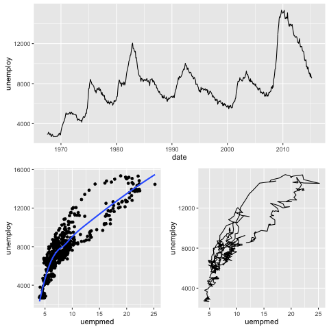
a <- qplot(date, unemploy, data = economics, geom = "line")
b <- qplot(uempmed, unemploy, data = economics) + geom_smooth(se = F)
c <- qplot(uempmed, unemploy, data = economics, geom = "path")

<span style="font-family: Georgia, 'Times New Roman', 'Bitstream Charter', Times, serif; line-height: 1.5;">library(grid)
vp1 <- viewport(width = 1, height = 1, x = 0.5, y = 0.5)
vp1 <- viewport()

#vieport()函数可创建视图窗口，参数x,y,width,height控制视图窗口的大小和位置（ｘ，ｙ控制视图窗口的中心位置）。默认的测量单位是“ｎｐｃ”，范围从０到１。（０,０），代表左下角，（１,１）代表右上角，（０.５,０.５）代表视图窗口的中心。也可以用ｕｎｉｔ（２，＂ｃｍ＂）或ｕｎｉｔ（１，＂ｊｉｎｃｈ＂）这样的绝对单位。</span>

#只占了图形设备一半的宽和高的视图窗口， 定位在图形的中间位置located in

# the middle of the plot.
vp2 <- viewport(width = 0.5, height = 0.5, x = 0.5, y = 0.5)
vp2 <- viewport(width = 0.5, height = 0.5)

#一个2cm x 3cm 的视图窗口，定位在图形设备中心

vp3 <- viewport(width = unit(2, "cm"), height = unit(3, "cm"))

#在右上角的视图窗口

vp4 <- viewport(x = 1, y = 1, just = c("right", "top"))

处在左下角

vp5 <- viewport(x = 0, y = 0, just = c("right", "bottom"))
pdf("polishing-subplot-1.pdf", width = 4, height = 4)	subvp <- viewport(width = 0.4, height = 0.4, x = 0.75, y = 0.35)
b
print(c, vp = subvp)
dev.off()

注意需要使用ｐｄｆ（）或ｐｎｇ（）将图形存储在磁盘中，因为ｇｇｓａｖｅ（）只能存储一张图。

自动分区――grid.layout() 将三幅图形分置在一页上

pdf("polishing-layout.pdf", width = 8, height = 6)
grid.newpage()
pushViewport(viewport(layout = grid.layout(2, 2)))
vplayout <- function(x, y) viewport(layout.pos.row = x, layout.pos.col = y)
print(a, vp = vplayout(1, 1:2))
print(b, vp = vplayout(2, 1))
print(c, vp = vplayout(2, 2))
dev.off()

二、facet_grid

# The base plot
p = ggplot(mpg, aes(x=displ, y=hwy)) + geom_point()

# Faceted by drv, in vertically arranged subpanels
p + facet_grid(drv ~ .)

# Faceted by cyl, in horizontally arranged subpanels
 p + facet_grid(. ~ cyl)

# Split by drv (vertical) and cyl (horizontal)
p + facet_grid(drv ~ cyl)

定义每行每列图的个数

# These will have the same result: 2 rows and 4 cols
p + facet_wrap( ~ class, nrow=2)
p + facet_wrap( ~ class, ncol=4)

每张子图的坐标系大小自定义

# The base plot
p = ggplot(mpg, aes(x=displ, y=hwy)) + geom_point()
# With free y scales
p + facet_grid(drv ~ cyl, scales="free_y")
# With free x and y scalesp + facet_grid(drv ~ cyl, scales="free")

改变子图的标签

mpg2 = mpg # Make a copy of the original data
 # Rename 4 to 4wd, f to Front, r to Rear
 levels(mpg2$drv)[levels(mpg2$drv)=="4"] = "4wd"
 levels(mpg2$drv)[levels(mpg2$drv)=="f"] = "Front"

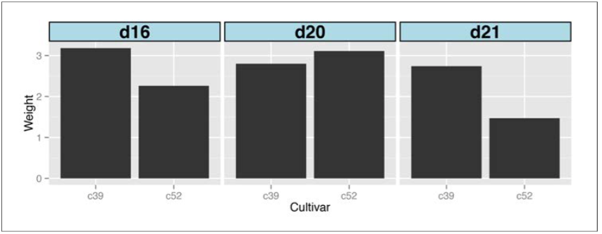
改变子图标签的背景色

library(gcookbook) # For the data set
ggplot(cabbage_exp, aes(x=Cultivar, y=Weight)) +geom_bar(stat="identity") +
facet_grid(. ~ Date) +
theme(strip.text = element_text(face="bold", size=rel(1.5)),
 strip.background = element_rect(fill="lightblue", colour="black",size=1))

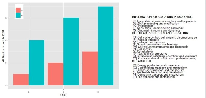
三、添加文字

a<-c("a","b","c");
b<-c(1,2,3);
c<-c(4,6,7);
abc<-data.frame(a,b,c);
abc;
 a b c
1 a 1 4
2 b 2 6
3 c 3 7

library(reshape2);
agcd<-melt(abc,id.vars="a",value.name="value",variable.name="bq");
text1<-read.delim("fun.txt",header=FALSE)
len<-nrow(text1);
a<-agcd[,1];
b<-agcd[,3];

library(ggplot2);
library(grid);
vp1<-viewport(width=0.6,height=1,x=0.3,y=0.5);
pm<-ggplot(agcd,aes(a,weight=value,fill=bq))+geom_bar(position="dodge")+theme(legend.title=element_blank(),legend.position=c(0.1,0.9))+xlab("COG")+ylab("M82/smithella and M82/SB");
 	 
#tiff(filename="haha.tif",width=25,height=12,units="cm",compression="lzw",bg="white",res=600)
png(file="aaaa.png",width=800,height=600);
par(fig=c(0.55,1,0,1),bty="n");
plot(1:b,1:b,type="n",xaxt="n",yaxt="n",xlab="",ylab="");#type="n"不生成任何点和线，为后面的命令创建坐标轴
 
sum=max(b)+b/(2*len);
 
for(i in 1:(len)){
 if (i %in% c(1,7,18,27) ){
text(1,sum,text1[i,],adj=0,cex=0.8,font=2);
 sum=sum-b/(len);
}else{
text(1,sum,text1[i,],adj=0,cex=0.8);
sum=sum-b/(len);}}
print(pm,vp=vp1);
dev.off();

参考资料：

ggplot2:数据分析与图形艺术